How a Neural Network Learns: Step-by-Step Breakdown from Zero

AI , Education
05 Apr, 2025

Inspired by the 3Blue1Brown series on neural networks. This article is a companion to the interactive neural network inspector, where you can step through every training epoch and examine every number inside.

What We’ll Build

Imagine you want to teach a computer to recognize handwritten digits 0, 1, and 2. Not through a pile of if statements and rules (“if the top-left pixels are lit — it’s a zero”), but through learning from examples — the way a child learns.

We’ll build the simplest possible neural network:

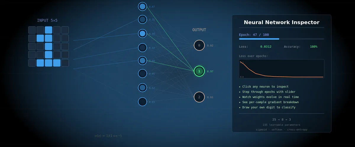
25 input neurons — each corresponds to one pixel of a 5×5 image
8 hidden neurons — “feature detectors” that learn to find patterns
3 output neurons — one for each digit (0, 1, 2)

A total of 235 parameters (weights and biases) that the network must tune on its own. This is a tiny network — for comparison, the network from the 3Blue1Brown video has 13,002 parameters, and GPT-4 has hundreds of billions. But the working principles are exactly the same.

🧪 Interactive inspector: Open the tool and set the epoch to 0. You’ll see the initial state of the network — random weights, uniform output distribution (~33% for each digit). The network knows nothing yet.

Part 1: What Is a Neuron

Forget biology. In our context, a neuron is a box that holds a number. This number is called the activation (denoted a), and it’s always between 0 and 1.

a = 0 — neuron is “off”, no signal
a = 1 — neuron is “fully on”, maximum signal
a = 0.73 — neuron is “partially active”

As Grant Sanderson (3Blue1Brown) puts it: “When I say ‘neuron’, all I want you to think of is ‘a thing that holds a number’.”

In the inspector, neurons are shown as circles on the graph. The brighter the circle — the higher the activation.

Input Neurons

Our 25 input neurons are simply the pixels of a 5×5 image. Each pixel has a value of 0 (black) or 1 (white). When we feed in an image of the digit “0”, some pixels = 1 (where the digit is drawn), others = 0 (background).

🧪 In the inspector: Hover over any input neuron. The tooltip will show: x[12] = 1 (pixel is on) or x[3] = 0 (pixel is off), along with a table of weights going from that pixel to each of the 8 hidden neurons.

Part 2: How Neurons Connect — Weights and Biases

Weights (`w`)

Every neuron in one layer is connected to every neuron in the next layer. Each such connection has a weight — a number that determines the strength and direction of the link.

Analogy: imagine a group of friends deciding where to have lunch. Each has their own preference — one really wants pizza (weight +0.8), another is firmly against sushi (weight -0.5), someone doesn’t care (weight ~0). The final decision is the sum of all “votes”, weighted by how strongly each person feels.

In our network:

Positive weight (+0.3) means: “if the input neuron is active, I also want to be active”
Negative weight (-0.5) means: “if the input neuron is active, I want to be less active”
Weight near zero (0.01) means: “I don’t care what this neuron does”

In the inspector, weights are shown as lines between neurons. Blue = positive weight, red = negative. Line thickness = connection strength.

Biases (`b`)

A bias is a neuron’s “sensitivity threshold”. Imagine the neuron is a judge at a competition. The bias determines how picky the judge is:

Negative bias (b = -2): “I’m hard to impress. The sum of signals must be really large for me to activate”
Positive bias (b = +1): “I’m easily impressed. Even a weak signal activates me”
Zero bias (b = 0): “I’m neutral”

Our network has 11 biases: one for each of the 8 hidden and 3 output neurons.

🧪 In the inspector: Hover over any hidden neuron — next to it you’ll see b=0.123. That’s the bias. At epoch 0, all biases = 0 (neutral). Scroll to epoch 50 — see how they’ve changed.

Part 3: The Forward Pass — How the Network Makes Decisions

The forward pass is the computation from input to output. Like a factory conveyor: raw material enters from one side, passes through several processing stations, and we get a finished product at the output.

Step 1: Weighted Sum

Each hidden neuron takes all 25 input values, multiplies each by its corresponding weight, and adds the results:

z = w₀×x₀ + w₁×x₁ + ... + w₂₄×x₂₄ + b

Where:

z — the “raw” sum, before activation. Can be any number: -5, 0, +12, whatever
w₀...w₂₄ — 25 weights for this neuron
x₀...x₂₄ — 25 pixel values (inputs)
b — bias

Concrete example. Suppose we feed in an image of digit “1” (a vertical line in the center). Pixels x₂, x₇, x₁₂, x₁₇, x₂₂ = 1 (center column), the rest = 0. Then:

z = w₂×1 + w₇×1 + w₁₂×1 + w₁₇×1 + w₂₂×1 + (rest × 0) + b
  = w₂ + w₇ + w₁₂ + w₁₇ + w₂₂ + b

Note: pixels with value 0 contribute nothing to the sum. Weight × 0 = 0, regardless of the weight. This is important for understanding why some weights don’t change when training on certain samples.

🧪 In the inspector: Click on hidden neuron h[0]. The tooltip will show the full calculation: z₁[0] = Σ(w·x) + b = 0.348 + (-0.127) = 0.221. Scroll down to the “Active connections (x>0)” table — every term is there.

Step 2: Activation Function — Sigmoid (σ)

The number z can be anything — from minus infinity to plus infinity. But we need an activation between 0 and 1. For this we use the sigmoid function, which 3Blue1Brown playfully calls “squishification”:

a = σ(z) = 1 / (1 + e^(-z))

What does it do? Squishes any number into the range (0, 1):

Input z	Output σ(z)	Interpretation
-5	0.007	Nearly off
-2	0.119	Weakly active
0	0.500	Neutral — right in the middle
+2	0.881	Strongly active
+5	0.993	Nearly fully on

Analogy: the sigmoid is a confidence meter. The number z is the neuron’s “raw score”. The sigmoid converts it to “confidence from 0 to 1”: how confident the neuron is that it detected its pattern.

Why not just clip? You could say: if z > 0, then a = 1, else a = 0. But a sharp boundary means a tiny change in z near zero can drastically change the output, while far from zero — nothing changes. The sigmoid is smooth instead — every change in z produces a proportional change in the output, which is critical for learning (gradients!).

Step 3: From Hidden Layer to Output

The process repeats: 3 output neurons take the 8 activations from the hidden layer, multiply by their weights, add biases… but instead of sigmoid, they use softmax.

Step 4: Softmax — Turning Numbers into Probabilities

Softmax is a way to convert 3 arbitrary numbers into 3 probabilities that sum to 1 (100%).

Suppose the 3 output neurons produced “raw” values:

z₂[0] = 2.1    (for digit 0)
z₂[1] = 0.5    (for digit 1)
z₂[2] = -0.3   (for digit 2)

Softmax does 2 steps:

Step A — raise e to the power of each number:

exp(2.1)  = 8.166
exp(0.5)  = 1.649
exp(-0.3) = 0.741

Why? Two reasons: (1) negative numbers become positive (you can’t have “negative probability”), (2) differences between numbers get amplified — the leader pulls further ahead.

Step B — divide each by the sum of all:

Sum = 8.166 + 1.649 + 0.741 = 10.556

P(digit 0) = 8.166 / 10.556 = 77.4%
P(digit 1) = 1.649 / 10.556 = 15.6%
P(digit 2) = 0.741 / 10.556 = 7.0%

The network thinks this is digit 0 with 77.4% confidence. The sum is always = 100%.

🧪 In the inspector: Click on any output neuron (digit 0, 1, or 2). The tooltip shows the full softmax calculation with all intermediate numbers: z₂, exp(z₂), sums, and the final percentage.

Interactive Neural Network Inspector

Part 4: Initialization — Where It All Begins

Before training, we need to set the initial values of all 235 parameters. This is a critical moment.

Why Not Start with Zeros?

If all weights = 0, then every neuron in the hidden layer computes the exact same number. And each receives the same gradient. And updates identically. Result: all 8 neurons remain identical forever — the network effectively has only 1 hidden neuron. It’s like a school where all students copy from each other — no diversity of knowledge.

He Initialization

We use the He method (Kaiming He, 2015): weights are drawn from a normal distribution with mean 0 and standard deviation √(2/n), where n is the number of inputs.

For our network:

W₁ (25→8): σ = √(2/25) ≈ 0.283 — weights will be small numbers roughly from -0.57 to +0.57
W₂ (8→3): σ = √(2/8) = 0.5 — weights are slightly larger because there are fewer inputs
All 11 biases start at 0

Why √(2/n) specifically? It’s a magic number chosen so that the signal neither vanishes nor explodes as it passes through layers. Too-small weights — the signal decays to zero. Too-large weights — numbers blow up to infinity. He initialization maintains the balance.

🧪 In the inspector: At epoch 0, look at the W₁ patterns in the right panel — 8 colored 5×5 grids. They look like random noise. Compare with epoch 100 — now each grid shows a clear pattern (horizontal lines, loops, vertical strokes).

Part 5: The Loss Function — Measuring How Wrong You Are

The network produced a prediction. But how good is it? For this we need a loss function — a numerical score of how far the prediction is from the correct answer.

Cross-Entropy

We use cross-entropy loss. The formula is simple:

L = -log(P_correct)

Where P_correct is the probability the network assigned to the correct digit.

Analogy: imagine a coach who doesn’t just count right/wrong answers, but evaluates confidence. If you correctly said “it’s digit 0” with 95% confidence — excellent, small penalty. But if you confidently (90%) said “it’s digit 1” while the correct answer is 0? Massive penalty!

Situation	P_correct	Loss = -log(P)	Rating
Confident and right	0.95	0.051	Excellent
Unsure but right	0.50	0.693	Average
Confident and WRONG	0.10	2.303	Bad!
Very confident and WRONG	0.01	4.605	Catastrophe!

Notice the nonlinearity: the difference between 0.95 and 0.50 is +0.642 in loss. But the difference between 0.10 and 0.01 is +2.302! Being confidently wrong is far worse than being uncertainly wrong. This is “how surprised the network is when it learns the truth.”

🧪 In the inspector: Loss is shown in the left panel as a number (e.g., loss=1.099) and a chart. At epoch 0, loss is 1.099 — the theoretical value for random guessing among 3 choices (-ln(1/3)). At epoch 100, loss is 0.001 — the network is nearly perfect.

Part 6: Gradient Descent — How the Network Learns

Now we know the network is making mistakes, and we can measure how badly (loss). The question: how do we change 235 parameters so the error decreases?

Analogy: Blindfolded on a Mountain

Imagine you’re standing on a mountain blindfolded. Your goal — descend into the valley (minimum loss). You can’t see anything, but you can feel the slope of the ground under your feet. The strategy is simple: take a step in the direction of steepest descent. Repeat.

In our case:

“Mountain” — the loss function as a function of 235 parameters
“Slope” — the gradient: a vector of 235 numbers, each telling how changing the corresponding parameter affects the loss
“Step” — updating all parameters simultaneously

The Gradient — Direction of Steepest Ascent

The gradient is a set of partial derivatives, one for each parameter. Each partial derivative ∂L/∂w says:

“If you increase this weight by a tiny number ε, the loss will change by (∂L/∂w) × ε.”

∂L/∂w > 0: increasing the weight increases loss — decrease the weight
∂L/∂w < 0: increasing the weight decreases loss — increase the weight
∂L/∂w ≈ 0: this weight barely affects loss — don’t bother

Grant Sanderson suggests thinking about the gradient not as a direction in space, but as an importance ranking: “which changes will have the biggest effect for the least effort.”

The Update Rule

w_new = w_old − lr × gradient

Where:

w_old — current parameter value
lr (learning rate) — a hyperparameter (a number set by a human, not the network). In our case lr = 1.2. Determines the step size
gradient — partial derivative of loss with respect to this parameter

The minus sign — because the gradient points in the direction of loss increase, and we want decrease.

Learning Rate — Step Size

Why lr = 1.2, and not 100 or 0.001?

Too large lr: steps are too big, you overshoot the valley floor, bouncing back and forth, never settling
Too small lr: tiny steps, training takes thousands of epochs
Right lr: big enough steps for fast progress, small enough for stability

This is one of the most important hyperparameters. It’s tuned experimentally.

🧪 In the inspector: Click on any connection (line between neurons) at epoch > 0. The tooltip at the bottom shows the full calculation:
Σ(∂L/∂w) = 0.269
avg = Σ/N = 0.269/24 = 0.011
Δw = −lr × avg = −1.2 × 0.011 = −0.013
w_new = w_old + Δw = 0 + (−0.013) = −0.013
Hover over lr — you’ll see the explanation: “Learning rate = 1.2”.

Part 7: Backpropagation — Finding Who’s to Blame

We know we need the gradient — the partial derivative of loss with respect to every weight. But how do we compute it? From loss to a specific weight is a long chain of computations. This is where backpropagation comes in.

The “Who’s to Blame?” Game

Imagine: the network saw digit 0 but answered “2” with 60% confidence. Someone is to blame. Backpropagation works like an investigation:

Step 1: Error at the output. Output neuron “digit 2” says: “I output 60%, but the correct answer is 0%. My error = 0.60 - 0 = +0.60”. Neuron “digit 0”: “I output 15%, but should have output 100%. Error = 0.15 - 1 = -0.85”. These differences (prediction − label) are denoted dz₂.

Step 2: Which hidden neurons are to blame? The error propagates back along connections. If the weight between h[3] and “digit 2” = +0.7, and the error of “digit 2” = +0.60, then h[3] receives “blame”: 0.7 × 0.60 = 0.42. Each hidden neuron receives the sum of blame from all three output neurons.

Step 3: The hidden neuron “filters” the blame. The hidden neuron multiplies the received blame by the sigmoid derivative σ'(z) = a × (1 - a). What does this mean?

If a ≈ 0.5 (neuron is unsure): σ’ = 0.5 × 0.5 = 0.25 — high value. The neuron is sensitive to changes, easily “persuaded”
If a ≈ 0.99 (neuron is very confident): σ’ = 0.99 × 0.01 = 0.0099 — nearly zero. The neuron is “stuck” and doesn’t want to change

This is the well-known vanishing gradient problem: neurons with very high or very low activations virtually stop learning.

Step 4: Weight updates. Now we know the gradient for every weight. For weight w₂[i][j] (from hidden j to output i):

∂L/∂w₂[i][j] = dz₂[i] × a₁[j]

That is: output error × hidden neuron activation. The logic: if the hidden neuron was very active (a₁ ≈ 1) and the output was wrong (dz₂ is large), then this weight is “guilty” — it needs a big change.

For first-layer weights w₁[j][k] (from input k to hidden j):

∂L/∂w₁[j][k] = dz₁[j] × x[k]

Where dz₁[j] is the hidden neuron’s “blame” (from step 3). Note: if x[k] = 0 (pixel is off), then gradient = 0, and this weight doesn’t change. This is logical: if the pixel wasn’t active, the weight from it couldn’t have affected the result, so there’s no point changing it.

The Chain Rule without Math

This entire process is the chain rule from calculus, but it has a simple intuition:

If changing weight W by a tiny amount changes neuron A by 3×, and changing A changes neuron B by 0.5×, and changing B changes loss by 2×, then the total effect of W on loss = 3 × 0.5 × 2 = 3.0.

Multiply effects at each step of the chain. That’s backpropagation — we go from the end (loss) to the beginning (weights) and at each step multiply the “local effect”.

🧪 In the inspector: Click on the connection between h[2] and output neuron “digit 0”. The tooltip shows:
∂L/∂w₂[0][2] = dz₂[0] × a₁[2]
dz₂ = a₂ − y (output error)
Below — a table with 24 samples: for each you can see a₂ (prediction), y (label), dz₂ (error), a₁ (hidden neuron activation), and the result ∂L/∂w.

Hover over any number in the dz₂ column — you’ll see the full computation chain, including where each component came from.

Part 8: Epoch vs Sample — The Rhythm of Learning

Now the most important distinction, one that’s often confused:

Within a Single Epoch

The network looks at each of the 24 training samples one by one. Weights and biases don’t change — they’re frozen. What changes are the neuron activations, because each sample has different input pixels.

But meanwhile, the network quietly accumulates complaints. For each sample, it computes a gradient: “this weight should be slightly larger”, “this bias is pointing the wrong way”. All these complaints add up.

Between Epochs

ONLY NOW do weights and biases change. The network takes the average of all 24 gradients and makes one update step. Then a new epoch begins — new frozen weights, go through all 24 samples again, collect new complaints, update.

Epoch 0:  random weights → run 24 samples → collect gradients → UPDATE weights
Epoch 1:  updated weights → run 24 samples → collect gradients → UPDATE weights
Epoch 2:  ...
...
Epoch 100: network is trained!

Analogy: it’s like a student who studies the entire textbook (= 1 epoch), then reviews their mistakes and corrects their understanding. Then re-reads the textbook — and understands more. Each pass = one epoch.

🧪 In the inspector: two sliders:

Epoch slider: changes which version of the brain you’re seeing (which weights/biases)

Sample slider: changes what this brain is looking at (which input is fed)

Fix epoch 1 and scroll through samples — see how the same weights produce different activations for different inputs. Then fix a sample and scroll through epochs — see how the weights change.

Part 9: What Happens During Training — Stage by Stage

Epoch 0: Chaos

Weights are random noise. Every neuron responds to an arbitrary set of pixels. Outputs — 33%/33%/33% — pure guessing. Loss — 1.099. Accuracy — 33%.

Epochs 1–3: First Steps

Gradients are largest — the network is far from the optimum. Weights make large jumps (Δw up to 0.05). Some neurons begin to “choose” a specialization — one responds more strongly to horizontal pixels, another to vertical ones.

Epochs 4–10: Rapid Learning

Clear patterns form. In the right panel, you can see W₁ grids transforming from noise into recognizable filters. Loss drops sharply. Accuracy jumps from 40% to 80%.

Epochs 11–30: Specialization

Every neuron has found its role. One detects the upper loop (characteristic of “0”), another — the vertical stroke (characteristic of “1”), a third — horizontal lines at the bottom (characteristic of “2”). Gradients decrease — the network approaches the optimum.

Epochs 31–60: Fine-Tuning

The big changes are behind. Now the network adjusts details — strengthening weights to distinguish similar cases (some variants of “0” look like “2”). Biases become important — they set the sensitivity threshold for each neuron.

Epochs 61–100: Convergence

Changes are minimal (Δw < 0.00001). Gradients are near zero. The network has reached a (local) minimum. Loss — 0.001. Accuracy — 100%. All 235 parameters are optimized.

🧪 In the inspector: Press ▶ Play and watch the entire transformation in real time. Follow the loss curve on the left — it draws the typical learning curve: flat at first (the network hasn’t found a direction yet), then a steep descent (found it!), then a gradual leveling off (reached the valley floor).

Part 10: Inference — Using the Trained Network

After 100 epochs of training, the weights are frozen forever. Now the network can recognize new digits it has never seen before.

Inference is simply a forward pass without learning:

Feed in 25 pixels of a new image
Compute weighted sums → sigmoid → weighted sums → softmax
Read the outputs: [85%, 10%, 5%] — “this is digit 0 with 85% confidence”

No gradients, no weight updates, no loss function. We simply apply the learned “rules” to new data. It’s like an exam after studying: the student (network) applies knowledge without feedback.

🧪 In the inspector: Switch to “Inference” mode. Draw a digit on the 5×5 canvas and watch the network process your input. Every neuron shows its activation, every connection — its weight. Click on any neuron — see the full forward pass calculation.

Variable Glossary

Symbol	Name	Meaning
`x[i]`	Input	Value of the i-th pixel (0 or 1)
`w₁[j][i]`	Layer 1 weight	Connection strength from input i to hidden neuron j
`b₁[j]`	Layer 1 bias	Sensitivity threshold of the j-th hidden neuron
`z₁[j]`	Weighted sum	w₁·x + b₁ — “raw” score before activation
`a₁[j]`	Activation	σ(z₁) — hidden neuron output (0..1)
`σ(z)`	Sigmoid	1/(1+e^(-z)) — squishes a number into (0,1)
`σ'(z)`	Sigmoid derivative	a×(1-a) — neuron’s sensitivity to changes
`w₂[i][j]`	Layer 2 weight	Connection strength from hidden j to output i
`b₂[i]`	Layer 2 bias	Sensitivity threshold of the i-th output neuron
`z₂[i]`	Output weighted sum	w₂·a₁ + b₂
`a₂[i]`	Softmax output	Probability that this is digit i (0..1, sum = 1)
`L`	Loss	-log(P_correct) — how badly the network erred
`∂L/∂w`	Gradient	Sensitivity of loss to changes in weight w
`dz₂[i]`	Output error	a₂[i] - y[i] — difference between prediction and label
`da₁[j]`	Back-propagated signal	Σ(w₂×dz₂) — “blame” from the output layer
`dz₁[j]`	Hidden gradient	da₁ × σ’ — blame accounting for sensitivity
`lr`	Learning rate	Training speed (hyperparameter, ours = 1.2)
`Δw`	Weight change	-lr × avg(gradient) — how much to shift the weight
`y[i]`	Label	Correct answer (1 for the correct digit, 0 for others)
`N`	Sample count	Number of training examples (ours = 24)

What’s Next?

This tiny 25→8→3 network illustrates all the key principles, but real networks have billions of parameters and more complex architectures. Here’s what changes at scale:

ReLU instead of sigmoid: max(0, z) — faster to compute and doesn’t have the vanishing gradient problem
Convolutional layers (CNN): instead of every neuron “seeing” all pixels, it sees only a small patch — more efficient for images
Dropout: during training, random neurons are “turned off” — forced diversity that prevents overfitting
Batch normalization: normalizing activations between layers for more stable training
Adam instead of plain gradient descent: adaptive lr for each parameter individually

But at the core of everything — the same 5 ideas: forward pass, loss function, backpropagation, gradient descent, iterative learning. Everything you saw in the inspector for 235 parameters scales to billions.

If you found this useful, consider supporting my work

Support on Patreon