Kalman Filters Explained: From Baby Steps to Black Magic

Engineering , Education
07 Apr, 2026

A companion guide to KalmanSim — no PhD required.

The Problem We’re Solving

Imagine you’re trying to find your cat in a dark apartment. You know roughly where she was five minutes ago (she was on the sofa). You also have a noisy sensor — your ears — that picks up faint rustling sounds, but you can’t tell exactly where the sound is coming from. Maybe it’s her, maybe it’s the fridge.

What do you do? You combine two imperfect pieces of information:

Your prediction — based on where she was, where she probably moved to
Your measurement — the noisy sensor reading right now

You don’t fully trust either one. You blend them together, weighted by how reliable each is. The more reliable your model of cat movement, the more you trust your prediction. The more reliable your ears, the more you trust the measurement.

That’s it. That’s the entire idea behind the Kalman filter.

The Kalman filter is a mathematically optimal way to do exactly this blending — and it keeps track of its own uncertainty as it goes. It knows when it’s confident and when it isn’t. And as we’ll see, different “flavors” of the filter exist because the world throws increasingly weird problems at us that break the simple version.

First, Some Vocabulary

Before we dive in, let’s agree on what the words mean.

Word	What it actually means
State	The thing you’re trying to estimate (position, velocity, temperature…)
Measurement	What your sensor actually reports — noisy, partial, sometimes wrong
Prediction	Where you think the state is, based on your model of how the world works
Update	Correcting your prediction using the measurement
Covariance	A fancy word for “how uncertain am I?” — a matrix that encodes your confidence
Innovation	The surprise — how different was the measurement from what you predicted?
Kalman Gain	How much should I trust this measurement vs my prediction? A number between 0 and 1

A high Kalman Gain means: trust the measurement more, I’m not very confident in my model. A low Kalman Gain means: ignore most of the measurement, my model is doing great.

The Core Loop: Predict → Measure → Update

Every single flavor of Kalman filter, no matter how exotic, follows the same three-step dance. Tattoo this on your brain:

   ┌──────────┐    ┌──────────────┐
   │ PREDICT  │───▶│    UPDATE    │
   └──────────┘    └──────────────┘
        ▲                │
        │                │
        └── new state ───┘
                ▲
          measurement

Step 1 — Predict: Use your model of the world to guess where the state is now, based on where it was. Also predict how uncertain you are.

Step 2 — Measure: Get a reading from your sensor. Compute the innovation — how surprised are you by this reading? Compute S, the total uncertainty of this innovation.

Step 3 — Update: Blend your prediction with the measurement. The blend ratio is the Kalman Gain, K. Update your uncertainty too — after seeing a measurement, you’re always at least a little more confident.

Then repeat. Every timestep. Forever.

The filter converges — meaning that over time, even starting with wild uncertainty, it homes in on the true state. This is one of the most beautiful properties in all of engineering.

Interactive simulator — KalmanSim

Part 1: The Linear Kalman Filter (LKF)

Also called: KF, Classical KF, Standard KF

The Assumption

The LKF is the elegant original from 1960, invented by Rudolf Kálmán while he was at NASA helping figure out how to navigate the Apollo spacecraft to the Moon. It works perfectly — and by perfectly I mean provably, mathematically optimally — under one key assumption:

Everything is linear, and all noise is Gaussian.

“Linear” means that if you double the input, you double the output. A rocket moving at 10 m/s for 1 second travels exactly 10 meters. Position after the next timestep is exactly old_position + velocity × dt. Simple, clean, linear.

“Gaussian” means the noise — both in your process and your sensor — follows a bell curve. No fat tails, no weird spikes, no systematic biases. Just random wobble centered on zero.

The Math, Gently

The state at time k is a vector x. For a simple 1D tracking problem: x = [position, velocity].

The filter needs you to specify four matrices upfront:

F — the transition matrix This encodes your model of how the state evolves. For constant velocity: if you were at position p with velocity v, next timestep you’re at p + v·dt with the same velocity v.

F = | 1   dt |
    | 0    1 |

Multiply F by your current state [p, v] and you get [p + v·dt, v]. That’s your prediction.

H — the observation matrix This encodes what your sensor actually measures. If your sensor only measures position (not velocity), then:

H = | 1   0 |

Multiplying H by the state [p, v] gives just p — the position — which is what gets compared to your measurement.

Q — process noise covariance How much does reality deviate from your model? Wind gusts? Unexpected acceleration? Q encodes your uncertainty about the model itself. Large Q = “I don’t trust my physics.” Small Q = “my model is excellent.”

R — measurement noise covariance How noisy is your sensor? A laser rangefinder has small R. A consumer GPS has large R. You usually get this from the sensor’s datasheet.

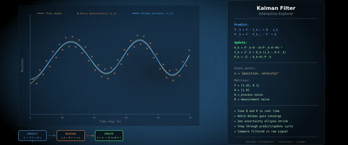
The Equations

Predict:

x⁻ = F · x            (predicted state)
P⁻ = F · P · Fᵀ + Q   (predicted covariance)

Measure:

y = z − H · x⁻        (innovation: how surprising is the measurement?)
S = H · P⁻ · Hᵀ + R   (total innovation uncertainty)

Update:

K = P⁻ · Hᵀ · S⁻¹     (Kalman Gain)
x = x⁻ + K · y        (updated state)
P = (I − K·H) · P⁻    (updated covariance)

That’s it. Eleven lines of math. Six equations. The foundation of an entire engineering discipline.

The Kalman Gain, Intuited

K is the magic. Look at the update equation: x = x⁻ + K · y.

If K = 0, the measurement is completely ignored. The filter trusts its prediction fully.
If K = 1 (simplified), the filter throws away its prediction and just uses the measurement.
Usually K is somewhere in between.

K → 0 happens when the measurement noise R is enormous (sensor is garbage) or when P⁻ is tiny (the filter is very confident already).

K → 1 happens when the measurement noise R is tiny (perfect sensor) or when P⁻ is huge (the filter is totally lost).

The filter automatically finds the right balance. This is why it’s “optimal” — given your stated assumptions about Q and R, no other linear estimator can do better.

When Does LKF Shine?

Tracking a boat at sea — roughly constant velocity, GPS measurements
Estimating room temperature — slow drift, thermometer noise
Smoothing a signal — noisy voltage readings from a sensor
Dead reckoning — combining accelerometer and position fixes
Any system where the physics is genuinely linear

When Does LKF Fail?

The moment your system becomes nonlinear, the LKF starts to struggle. And it fails silently — the numbers still come out, they’re just wrong. No error message. No warning. Just subtly diverging estimates.

Examples of nonlinearity that break LKF:

Radar bearing measurements — range and bearing to a target involve arctangent and distance, which are nonlinear
Coordinated turns — a plane banking involves trigonometric relationships
Gravity on a pendulum — the restoring force is sin(θ), not θ
Robot with wheel odometry — heading integrates nonlinearly into position

Enter the extended filter.

Part 2: The Extended Kalman Filter (EKF)

The workhorse of aerospace, robotics, and navigation

The Core Idea

The EKF’s answer to nonlinearity is wonderfully pragmatic: linearize at each step.

Instead of requiring linear functions everywhere, the EKF says: “OK, the true function is curved. But if I’m close enough to the current estimate, I can approximate it as locally linear using a Taylor expansion.” It computes the Jacobian — the matrix of first derivatives — at the current operating point, and uses that as if it were the F matrix.

It’s like navigating by drawing a straight line that’s tangent to the curve right where you’re standing. Not perfect, but pretty good if you’re updating frequently enough.

The New Ingredients

Now the state dynamics and measurement functions can be arbitrary nonlinear functions:

x(k+1) = f(x(k), u(k)) + noise   (process model, now nonlinear)
z(k)   = h(x(k)) + noise         (measurement model, now nonlinear)

Where f and h are potentially any functions you can write down.

The trick: replace F and H with their Jacobians, evaluated at the current estimate:

F_jacobian = ∂f/∂x evaluated at x = x̂
H_jacobian = ∂h/∂x evaluated at x = x̂

A Jacobian is just a matrix of partial derivatives — each entry tells you “how much does output i change if I nudge input j?”

Worked Example: Radar Tracking

You’re tracking a plane with a radar dish. Your state is [x_position, y_position, x_velocity, y_velocity].

Your measurement is [range, bearing] — the distance and angle to the plane. These are computed as:

range   = √(x² + y²)
bearing = atan2(y, x)

Neither of those is linear in [x, y]. But the EKF can still handle it. The Jacobian of h with respect to [x, y] is:

∂range/∂x   =  x / √(x² + y²)
∂range/∂y   =  y / √(x² + y²)
∂bearing/∂x = −y / (x² + y²)
∂bearing/∂y =  x / (x² + y²)

Evaluated at the current estimate, this gives a local linear approximation that the filter uses just like H in the LKF.

When EKF Shines

GPS/INS navigation — combining inertial measurements with GPS fixes, highly nonlinear state transitions
Simultaneous Localization and Mapping (SLAM) — robots building maps while navigating them
Spacecraft attitude estimation — quaternion dynamics are nonlinear
Sensor fusion with bearings-only measurements — range-free radar, acoustic arrays
Any system that’s mildly-to-moderately nonlinear

The EKF is the de facto standard in aviation, missiles, and spacecraft. The Apollo Guidance Computer used something very close to an EKF. It’s running in your phone’s GPS chip right now.

When EKF Fails

The EKF has three Achilles heels:

1. Strong nonlinearity. If the function curves sharply, the linear approximation is terrible. Imagine approximating a hairpin turn with a straight line — you’ll drive off the road. The EKF diverges (estimates blow up or become nonsense) in highly nonlinear regimes.

2. You have to compute the Jacobian by hand (or use auto-differentiation). For complex systems, deriving ∂f/∂x analytically is painful and error-prone. Get one sign wrong and the filter gives subtly wrong answers forever. This is a real engineering hazard.

3. Non-Gaussian noise gets mangled. Passing a non-Gaussian distribution through a nonlinear function creates a more non-Gaussian distribution. The EKF approximates it as Gaussian anyway. For mildly non-Gaussian cases this is fine. For heavy-tailed or multimodal distributions, it’s a disaster.

When the EKF fails, you have two better options.

Part 3: The Unscented Kalman Filter (UKF)

Smarter than EKF, requires no derivatives

The Insight

Jeffrey Uhlmann, a computer scientist, asked a provocative question in 1994: Is it really true that it’s easier to approximate a distribution than to approximate a nonlinear function?

His answer was: no, it’s the other way around. This became the Unscented Transform, the heart of the UKF.

It’s easier to approximate a probability distribution than to linearize a function.

Instead of linearizing the function f and propagating a Gaussian through the approximation, the UKF propagates a carefully chosen set of sample points — called sigma points — directly through the true nonlinear function f, and then reconstructs the output statistics from those propagated points.

No Jacobians. No derivatives. No linearization.

The Unscented Transform

Given a Gaussian distribution with mean x and covariance P, the Unscented Transform picks 2n+1 sigma points (where n is the state dimension):

χ₀ = x                                  (the mean itself)
χᵢ = x + (√((n+λ)P))ᵢ      for i=1..n   (spread in positive direction)
χᵢ = x − (√((n+λ)P))ᵢ₋ₙ    for i=n+1..2n (spread in negative direction)

Where λ is a tuning parameter controlling how far out the sigma points are spread.

Each sigma point has an associated weight — the central point gets more weight, the outer points get less. The weights sum to 1.

Then you push each sigma point through the nonlinear function f:

γᵢ = f(χᵢ)   for each sigma point

Finally, you reconstruct the output statistics from the transformed sigma points:

x⁻ = Σ Wᵢ · γᵢ                            (weighted mean = predicted state)
P⁻ = Σ Wᵢ · (γᵢ − x⁻)(γᵢ − x⁻)ᵀ + Q       (predicted covariance)

The rest of the filter (measurement update, Kalman gain computation) works exactly the same as LKF/EKF.

Why Is This Better Than EKF?

The magic is in the accuracy of the approximation. The UKF captures the true mean and covariance of the transformed distribution to second order (technically third order for symmetric distributions). The EKF only captures them to first order — that’s why it struggles with strong nonlinearity.

Think of it this way:

EKF: draws one tangent line at the current point and uses that line everywhere
UKF: picks a handful of points that perfectly capture the shape of your uncertainty, pushes them all through the real function, and sees where they land

The UKF is almost always more accurate than the EKF. The price you pay is slightly more computation (2n+1 function evaluations instead of 1), and you need to tune a handful of extra parameters (α, β, κ that control sigma point placement).

Worked Example: The Pendulum

A pendulum’s equation of motion is:

θ̈ = −(g/L) · sin(θ)

That sin(θ) is deeply nonlinear. For small angles, sin(θ) ≈ θ, so LKF works fine. For large swing angles (say, 90°), the approximation is terrible — sin(90°) = 1.0 but 90° in radians ≈ 1.57. The LKF thinks it’s 57% more restoring force than there actually is.

The EKF linearizes sin(θ) as cos(θ₀), which is slightly better but still an approximation that degrades at large angles.

The UKF sends sigma points at angles like [θ−Δ, θ, θ+Δ] all through the real sin() function, sees exactly where they land, and correctly captures the nonlinear distortion. It handles this scenario with grace where EKF starts to struggle.

UKF Tuning Parameters

The UKF has three tuning knobs:

Parameter	What it does	Typical value
α	Controls spread of sigma points	1e-3 to 1
β	Encodes prior knowledge about distribution shape (2 = Gaussian)	2
κ	Secondary scaling (often 0 or 3−n)	0

From these, λ = α²(n+κ) − n. Getting these wrong can make the filter worse than EKF, so tuning matters.

When UKF Shines

Attitude estimation — quaternion kinematics are strongly nonlinear; UKF handles gimbal-lock-adjacent regimes where EKF diverges
Chemical process control — reaction kinetics are often highly nonlinear
Finance — stochastic volatility models (yes, Kalman filters are used in quantitative finance)
Any time you can’t derive the Jacobian analytically — just code f() and let the UKF figure it out
When EKF is diverging and you need a drop-in replacement

When UKF Falls Short

Very high-dimensional state spaces — the 2n+1 sigma points become expensive for n ≥ 100
Highly non-Gaussian distributions — if your true posterior is bimodal or heavily skewed, both EKF and UKF fail; you need particle filters
Computational constraints — embedded systems where even 2n+1 function evaluations per step is too expensive

Part 4: Other Nonlinear Filters Worth Knowing

Before we get to IMM, a brief tour of the wider landscape.

The Cubature Kalman Filter (CKF)

A close cousin of the UKF, proposed in 2009. Instead of the sigma-point rules above, it uses a specific set of 2n cubature points uniformly distributed on a sphere. Claimed to be numerically more stable than UKF in high dimensions. Used in GPS-aided INS systems for aircraft and satellites.

The Particle Filter (PF)

When Gaussian assumptions completely break down — think tracking a person in a building where they could be in any of five corridors — the particle filter is the answer. Instead of maintaining a mean and covariance, it maintains thousands of “particles” (hypotheses) each with a weight representing how likely it is.

Pros: Handles any distribution, handles multimodal posteriors, handles severe nonlinearity
Cons: Extremely computationally expensive (thousands of samples per step), suffers from “particle degeneracy” (most weights shrink to zero after a few steps without resampling tricks)

The particle filter is the theoretically correct solution to arbitrary Bayesian estimation. Every other filter on this page is an approximation of the particle filter.

The Square Root Kalman Filter

Not a different algorithm, but a numerically stable implementation of the KF/EKF/UKF. Instead of storing P directly, it stores its Cholesky factor (the square root). This prevents the covariance matrix from becoming non-positive-definite due to floating point errors — a real problem in 32-bit embedded implementations.

Used extensively in aerospace where numerical stability is a safety requirement.

The Information Filter

Mathematically equivalent to the KF, but parameterized by the information matrix (inverse of covariance) and information vector. Initialization with complete ignorance (P → ∞) becomes trivial (information = 0). Useful in distributed sensor fusion where multiple agents share information updates.

Part 5: The Interacting Multiple Model Filter (IMM)

For when you don’t know which model is correct — so you run all of them simultaneously

The Motivation

All the filters above assume you know which model describes your system. But what if you don’t?

Consider tracking a fighter jet:

Sometimes it flies straight (constant velocity model)
Sometimes it executes a coordinated turn (constant turn-rate model)
Sometimes it dives or climbs (vertical maneuver model)

You don’t know which mode it’s in. A single-model filter will:

Lag behind during maneuvers if it’s tuned for straight flight
Be jittery during straight flight if it’s tuned for aggressive maneuvers

The IMM solves this by running multiple models simultaneously and mixing their outputs based on how well each model explains the current measurements.

It’s like having three detective friends, each specializing in a different scenario. You listen to all of them, but weight their opinions by how well their predictions have been matching reality lately.

The Architecture

┌─────────────────────────────────────────────────┐
│                   IMM FILTER                    │
│                                                 │
│   ┌─────────┐   ┌─────────┐   ┌─────────┐       │
│   │ Model 1 │   │ Model 2 │   │ Model 3 │       │
│   │  (LKF)  │   │  (EKF)  │   │  (UKF)  │       │
│   └────┬────┘   └────┬────┘   └────┬────┘       │
│        │             │             │            │
│        └─────────────┴─────────────┘            │
│                      │                          │
│               ┌──────┴──────┐                   │
│               │   MIXING    │                   │
│               │  (weights)  │                   │
│               └──────┬──────┘                   │
│                      │                          │
│               ┌──────┴──────┐                   │
│               │   OUTPUT    │                   │
│               │  ESTIMATE   │                   │
│               └─────────────┘                   │
└─────────────────────────────────────────────────┘

The Four Steps of IMM

Step 1 — Model interaction (mixing). Each model receives a “mixed” initial state, computed as a weighted combination of all models’ current estimates. The weights come from the probability that each model is active, multiplied by the transition probability between models. This mixing step is what makes IMM “interacting” rather than just “parallel filters.”

Step 2 — Mode-conditioned filtering. Run each filter independently with its mixed initial state. Each produces an updated estimate and covariance.

Step 3 — Mode probability update. Update the probability that each model is active, based on the likelihood of the current measurement given each model’s predictions.

If Model 1 (straight flight) predicted the plane would be at [100, 200] and the radar says it’s at [100, 205], Model 1 gets rewarded. If Model 2 (turning) also predicted [100, 205], they get equal credit.

The likelihood function for Gaussian noise is:

Λᵢ = (1 / √(2π|Sᵢ|)) · exp(−0.5 · yᵢᵀ · Sᵢ⁻¹ · yᵢ)

where yᵢ is the innovation for model i and Sᵢ is the innovation covariance.

Step 4 — Output fusion. The final estimate is the probability-weighted average of all models’ estimates:

x̂ = Σ μᵢ · x̂ᵢ
P  = Σ μᵢ · [Pᵢ + (x̂ᵢ − x̂)(x̂ᵢ − x̂)ᵀ]

where μᵢ is the current probability of model i.

The Transition Probability Matrix

One input you must provide to IMM is the Markov transition matrix — how likely is it that the system switches from mode i to mode j in one timestep?

For a 3-mode tracker:

              from straight   from turning   from climbing
to straight:  [    0.90           0.05           0.05    ]
to turning:   [    0.05           0.90           0.05    ]
to climbing:  [    0.05           0.05           0.90    ]

This says: whatever mode the target is in, it stays in that mode 90% of the time and transitions to any other mode 5% of the time. Real aircraft have different values tuned empirically.

What Makes IMM Special

Automatic mode detection: the model probabilities μᵢ tell you what the system is doing right now. If μ₂ (turning model) spikes to 0.9, the aircraft is turning. This is genuinely useful information.
Smooth transitions: there’s no sudden “switch” between models. The output smoothly transitions as the probabilities evolve.
Bounded computation: unlike a particle filter, IMM has fixed computational cost (one filter per model per timestep).
Any mix of filter types: Model 1 can be LKF, Model 2 EKF, Model 3 UKF. Whatever fits each mode.

Classic IMM Scenarios

Maneuvering target tracking — the original application. Three models: constant velocity, constant turn rate, constant acceleration. Used in air traffic control radar processors, military tracking systems, and missile guidance.

Vehicle tracking on roads — straight driving (LKF), turning at intersection (EKF with turn-rate state), reversing (different model). Used in automotive ADAS systems.

Fault detection — Model 1 is normal operation, Model 2 is sensor-failed state. If the probability of Model 2 climbs, a fault has occurred. The IMM becomes a real-time fault detector.

Structural health monitoring — a bridge that switches between normal flexing and damaged-flexing modes. IMM detects structural changes over time.

Limitations of IMM

Model set must cover reality: if the true mode isn’t in your set, the filter will do its best with what it has — often spreading weight across the closest models, giving a mushy answer.
Transition matrix is hard to tune: wrong transition probabilities lead to slow mode switching (too high diagonal) or jittery mode changes (too low diagonal).
Grows with number of models: 10 models means 10 parallel filters and O(10²) mixing computations.
Still assumes Gaussian within each mode: if each individual mode has non-Gaussian noise, you’d need particle filters within each mode.

Comparison Table

Property	LKF	EKF	UKF	IMM
Handles nonlinearity	✗	✓ (mild–moderate)	✓ (moderate–strong)	✓ (depends on sub-filters)
Jacobians required	✗	✓ (you must derive)	✗	depends
Computational cost	low	low	medium (2n+1 evals)	medium–high (per model)
Handles multiple modes	✗	✗	✗	✓
Optimal for linear/Gaussian	✓	✗	✗	✗
Accuracy (nonlinear)	poor	moderate	good	good (per mode)
Numerical stability	good	can diverge	generally good	generally good
Tuning complexity	low	medium	medium	high
Earliest use	1960 (Apollo)	1960s (aerospace)	1994 (robotics)	1988 (tracking)

Decision Guide: Which Filter to Use?

Is your system linear (or close enough)?
├── Yes → Use LKF. It's optimal. Don't overcomplicate it.
└── No  → Is the nonlinearity mild? (smooth functions, small angles, slow dynamics)
    ├── Yes → Try EKF first. Simple, fast, usually good enough.
    │         └── Diverging or inaccurate? → Switch to UKF.
    └── No  → Use UKF. Skip EKF entirely.
              └── Highly non-Gaussian / multimodal?
                  └── Yes → Use a Particle Filter.

Does your system switch between different dynamic regimes?
└── Yes → Wrap whatever filter(s) above in an IMM.

The Matrices: A Deeper Look

Every Kalman filter variant is essentially a story told through matrices. Let’s build some intuition.

Q — process noise: “How much do I trust my model?”

Q = | σ²_pos    0    |
    |   0    σ²_vel  |

Large Q diagonal: “My physics model is rough. Maybe there’s wind, friction, unknown forces. Expect reality to deviate from my prediction.” → Filter trusts measurements more, responds faster to changes, but noisier estimates.
Small Q diagonal: “I know this system’s dynamics precisely. A thrown ball follows the parabola, period.” → Filter trusts predictions more, smoother estimates, but slow to respond to unexpected maneuvers.
Off-diagonal entries in Q: If position error and velocity error are correlated (a fast target tends to have position errors in the direction of motion), off-diagonal terms capture this. Often set to zero for simplicity.

Tuning tip: Start with Q = σ²_model · I and tune from there. If estimates are too smooth and lag real movements, increase Q. If estimates are too noisy, decrease Q.

R — measurement noise: “How much do I trust my sensor?”

R = | σ²_sensor |    (1D case)

This one’s usually easiest to specify — it comes from the sensor’s datasheet or from calibration experiments. Put a sensor in front of a known target, record 1000 measurements, compute the variance. That’s your R.

Large R → Kalman Gain K is small → measurements barely influence the estimate → smooth but slow
Small R → Kalman Gain K is large → measurements dominate → noisy but responsive

P — state covariance: “How uncertain am I right now?”

P evolves dynamically. You initialize it with P₀ (your initial uncertainty about the state), and the filter updates it every step.

P₀ = | 100    0  |    (very uncertain about initial position and velocity)
     |   0  100  |

After many updates, P typically shrinks as the filter becomes more confident. The diagonal entries tell you the variance of each state variable. The off-diagonal entries tell you how correlated your estimates are (e.g., if you’re uncertain about position, are you also uncertain about velocity in the same direction?).

The covariance P is the filter’s “confidence score”. Watch it decrease over time as the filter accumulates evidence. If it starts growing, something is wrong — your model is diverging.

Common Failure Modes (and How to Debug Them)

Filter Divergence

Symptoms: Covariance P blows up to infinity, estimates fly off to nonsensical values. Causes: Q or R set to zero (numerical singularity), model is too wrong, strong nonlinearity exceeding EKF’s range. Fix: Check Q > 0, increase Q, switch to UKF.

Filter Overconfidence

Symptoms: P is tiny but errors are large. The filter “thinks” it knows exactly where the target is, but it’s wrong. Causes: Q too small (filter trusts its model too much and ignores measurements), or the process noise is actually much larger than modeled. Fix: Increase Q.

Innovation Growing

Symptoms: The innovations (y = z − H·x⁻) are getting larger over time rather than staying near zero. Causes: The model is drifting from reality — either the dynamics model is wrong, or there’s a sensor bias you’re not modeling. Fix: Check that the innovation is zero-mean. Add a bias state to the filter. Increase Q.

Noisy Estimates

Symptoms: Output estimate jumps around — more noisy than the raw measurements. Causes: Q too large (filter doesn’t trust its model), R too small (filter over-weights noisy measurements). Fix: Decrease Q, or increase R.

IMM Model Weights All Equal

Symptoms: All model probabilities μᵢ hover near 1/N. The IMM can’t determine which model is active. Causes: The models are too similar (they predict nearly the same things), or the measurement noise R is so large that the likelihoods are indistinguishable. Fix: Make models more distinct, reduce R, or add more discriminative measurements.

Historical Context: How We Got Here

1960 — Rudolf Kálmán publishes “A New Approach to Linear Filtering and Prediction Problems” in the ASME Journal. NASA immediately recognizes its importance. Kálmán visits the Ames Research Center, and the filter is implemented for the Apollo navigation computer.

1960s–1970s — The EKF is developed in the aerospace community as engineers tackle the nonlinear navigation problems of missiles and spacecraft. Attribution is diffuse — many engineers independently developed similar ideas.

1988 — The IMM concept (in its modern form) is published by Blom and Bar-Shalom in the context of maneuvering target tracking for air traffic control radars.

1994 — Jeffrey Uhlmann proposes the Unscented Transform as part of his PhD research at Oxford. Simon Julier and Uhlmann publish the UKF in 1997.

Late 1990s — The particle filter gains traction with falling compute costs. It had been theoretically understood for decades but was too expensive to run in real-time.

2000s — Kalman filters become ubiquitous in consumer devices. Your phone’s GPS uses them. The accelerometer in your AirPods uses them to detect your head position. The autopilot on commercial flights uses them continuously.

Today — Neural-network–Kalman-filter hybrids emerge, where the process model f or measurement model h is a learned neural network rather than a hand-derived physics equation.

What This Simulator Shows You

KalmanSim walks you through the core LKF loop step by step, making each mathematical operation visible:

Predict step: watch x⁻ and P⁻ computed in real time, see how the uncertainty grows during prediction
Measure step: see the innovation y and how it depends on how surprising the measurement is
Update step: watch the Kalman gain K balance prediction vs measurement, and see P shrink after an update

The matrix heatmaps reveal structure that’s invisible in raw numbers — you can see P start diagonal and develop off-diagonal correlations as position and velocity estimates become coupled.

By tuning Q upward, you can watch the filter become “nervous” — trusting measurements more, tracking faster but with more noise. Tune Q down and watch it become “stubborn” — smooth estimates that lag sudden changes.

EKF, UKF, and IMM are coming to KalmanSim next. Each will demonstrate scenarios where LKF breaks, and show how the more advanced filter handles what LKF cannot.