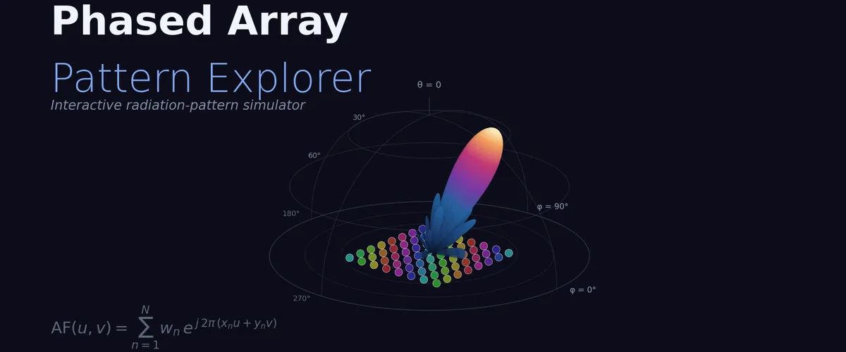
Phased Array Pattern Explorer

Phased arrays are everywhere now — 5G base stations, satellite terminals, automotive radar, every mmWave system worth building. The math behind them is gorgeous: a sum of plane waves from N elements, each with its own phase and amplitude, producing a directional beam you can electronically steer without moving a single mechanical part. But the elegance hides a lot of practical machinery — tapers, grating lobes, beamwidth scaling, phase quantization, frequency squint — and reading about it is no substitute for seeing what changes when you move a slider.

So I built the playground I wished I’d had when I was learning this material. It runs in the browser, no install, no MATLAB licence. Pick a geometry, set the element count and spacing, choose a taper, aim the beam, and the simulator computes the radiation pattern in real time.

What’s in it

Four geometries: linear (1‑D), rectangular (N_x × N_y), circular ring, and hexagonal lattice. Same array‑factor sum under the hood — only the element positions differ.

Eight tapers: uniform, triangular, cosine, Hamming, Hann, Blackman, Taylor (−25 dB), Dolph‑Chebyshev (−30 dB). The classic sidelobe‑vs‑beamwidth trade‑off is right there in the metrics panel. Chebyshev’s equiripple sidelobes are mesmerising on the polar plot.

Five element patterns: isotropic, cosine, sin θ, half‑wave dipole, microstrip patch — multiplied with the array factor for the realistic total pattern.

Four visualisations: polar plot, Cartesian dB cut, U‑V (k‑space) heatmap, and a full 3‑D surface in Three.js with the steered beam shown as an arrow. Each view tells you something different — the polar gives instant beamwidth intuition, the Cartesian quantifies SLL, the U‑V map shows you grating lobes outside the unit disc, and the 3‑D shows the full hemispheric pattern.

The wrinkles that ruin real arrays

Beyond the textbook case, the simulator includes the impairments that nobody warns you about until you build one:

• Phase‑shifter quantisation at 1–8 bits — drop to 2 bits and watch quantisation lobes erupt out of nowhere.
• Gaussian phase and amplitude errors with seeded reseed for reproducibility.
• Element failures — click any element on the layout view to kill it and watch the pattern degrade.
• Frequency squint — slide Δf/f₀ and compare phase‑shifter against true‑time‑delay beamformers. The beam wanders in one mode, stays put in the other.

A few things to try

• Crank element spacing to 0.9 λ and watch grating lobes drift in from the horizon.
• Steer a 32 × 32 array to 60° with 2‑bit phase quantisation. It’s a beautiful disaster.
• Pick the hex preset with four rings and notice how circular symmetry softens grating lobes compared to a rectangular grid.
• Switch from a uniform taper to Chebyshev at the same SLL — same sidelobe floor costs you ~15% extra beamwidth.

Every slider has a KaTeX‑rendered formula explaining the math behind it. The point isn’t to replace a proper EM simulator; it’s to give you the intuition a paper can’t.

---