Three modes, one resonator: an interactive DRA explorer

The dielectric resonator antenna (DRA) is one of those antenna types you keep meeting if you work in RF: 5G handsets, automotive radar modules, GPS pucks, satellite comms terminals. And yet most introductions stop at “it’s a small ceramic chunk that radiates.” Which is technically true, and almost entirely useless.

The reason DRAs are hard to teach is that the interesting things happen in three dimensions: standing waves form inside the dielectric, the mode you excite depends on how you feed it, and the size–bandwidth tradeoff is sharp enough to design careers around. None of that survives on a textbook page.

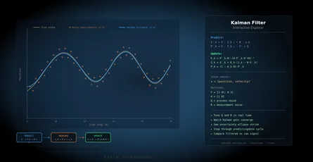
The widget below is a live DRA mode visualizer — change the geometry and watch what happens. The rest of the post is a short guide to what you’ll see.

What is a DRA, anyway?

Take a chunk of high‑permittivity ceramic — εᵣ somewhere between 10 and 100 — and sit it on a metal ground plane. The boundary between ceramic and air reflects waves back inside (low permittivity acts like an “imperfect mirror”), and the metal ground reflects them too. You get a 3D resonator: standing electromagnetic waves at specific frequencies, just like a Helmholtz resonator for sound.

Unlike a Helmholtz resonator, this one radiates. The imperfect air boundary lets a small fraction of the stored energy leak out into a far‑field pattern. Tune the geometry and you tune the radiation pattern, the frequency, and the bandwidth.

Three canonical modes

For a cylindrical DRA on a ground plane, three lowest‑order modes do almost all the practical work:

• TE₀₁δ — closed E‑field loops circulating in horizontal planes, vertical H on the axis. Radiates like a short vertical magnetic dipole: omnidirectional in azimuth, null overhead, max near the horizon. Horizontal polarization.
• HE₁₁δ — hybrid mode with cos(φ) angular dependence. Behaves like a short horizontal magnetic dipole plus its image, giving strong broadside (overhead) radiation. The closest DRA cousin of a microstrip patch antenna and the workhorse for mobile/wireless.
• TM₀₁δ — vertical E‑lines arch over the top of the resonator and return to ground at the rim. Same pattern as a short vertical monopole — vertical polarization, omni in azimuth, null overhead.

In the tool, click the small i next to each mode for a full intuition brief: physical analog, radiation pattern, polarization, excitation methods, and applications.

The aha: εᵣ trades size for bandwidth

This is the lesson the tool is built to deliver. Drag the εᵣ slider.

At εᵣ = 10 the DRA is comfortably large for its frequency, and the bandwidth sits around 9–10 %. Crank the slider to εᵣ = 100 and the same antenna shrinks to about a fifth the diameter — but bandwidth collapses below half a percent. Q‑factor explodes, the resonance becomes a thin spike, and manufacturing tolerances drop into the sub‑millimeter range.

This isn’t a flaw. It’s the fundamental size–bandwidth tradeoff of any electrically small antenna, shown in its cleanest possible form. Watching it happen live, with the frequency and Q readouts updating in real time, is much more visceral than reading “Q ∝ εᵣ^1.27” in Petosa.

Feed position is more decisive than you’d think

Switch to HE₁₁δ and drag the feed‑position slider from the center toward the rim. The field nearly vanishes at the center and grows as you move outward — because HE₁₁δ has an E_ρ ∝ J₁(k_ρ ρ) component, and J₁(0) = 0. A vertical probe inserted at the center sees no field tangent to it. No coupling, no excitation.

Now switch to TE₀₁δ and try every feed position from 0 to 100 %. The field stays faintly visible everywhere. That’s the textbook fact made obvious: TE₀₁δ has no E_z component anywhere, so a vertical coaxial probe is blind to it. To launch this mode you need an aperture‑coupled slot in the ground plane or a side‑mounted strip. The tool shows you this instantly: η ≈ 0 % across the entire feed track.

What’s under the hood

Every visualization has the symbolic math sitting next to it: Mongia–Kishk resonance formulas for each mode, empirical Q‑factor expressions, bandwidth at VSWR = 2 — and a numeric substitution line showing the actual values plugged in for whatever geometry you’ve dialed in. The 3D scene shows oscillating field vectors (colored by polarity, length tracking instantaneous amplitude), a vertical slice plane with a viridis envelope heatmap, and a feed marker that lights up green/yellow/red with coupling efficiency.

For deeper reading, Petosa’s Dielectric Resonator Antenna Handbook is the standard reference. Long, McAllister and Shen’s 1983 paper is the original DRA proposal. And 3Blue1Brown’s videos on Bessel functions are a good warm‑up if any of the math above looked unfamiliar.

---